How we made continuous trace intelligence possible at scale

If you run an agent in production, some part of your day is probably going through the countless production logs to see if anything looks interesting. You know there's good intel in there somewhere, but the data doesn't tell you what question you should be asking, or what SQL query would capture it.

We've been thinking about this problem at Braintrust for a long time, and Topics is the solution that lets you analyze traces with intelligence at scale. Like Brainstore, it's one of the small number of big, concentrated technical bets we've made on owning a primitive end-to-end rather than stitching together off-the-shelf pieces. With Brainstore the bet was on the storage and query layer. With Topics, the bet is on the intelligence layer that sits on top.

What makes trace classification hard

In order to find patterns you didn't know to look for, you need to run this intelligence layer over every trace. We call this active observability. But exposing a coding agent to 100% of your production traffic is too expensive, so the job is to distill it down to the handful of things worth looking at. Cost stands in the way because LLM traces aren't shaped like anything the standard tools expect.

The standard NLP toolkit assumes documents that are roughly uniform in shape and size. Topic modeling with LDA wants bag-of-words documents in the hundreds of tokens. Sentiment analysis wants a sentence or a paragraph. Off-the-shelf clustering on embeddings wants inputs that fit inside an embedding model's context window, which today caps out around 8,192 tokens.

Agent traces don't look like that. A single production trace can be millions of tokens of conversation history, tool calls, intermediate reasoning, retrieved context, and serialized application state. They arrive at high volume, they keep updating after they're "done," and the interesting signal is usually buried in a few spans out of hundreds. If you embed the raw trace, you get noisy clusters dominated by surface features like message length or tool name frequency. If you summarize first with an LLM, you blow your budget. If you sample aggressively, you miss the long tail, which is where the bugs usually live.

There's also a methodology problem. Teams want to ask three different questions of the same logs: what kinds of requests are coming in, what's going wrong, and how do users feel about the responses? Those are usually three different stacks. Topic modeling for the first, error mining or anomaly detection for the second, and sentiment analysis for the third. Maintaining three pipelines, each with its own preprocessing and its own failure modes, is not a great use of an applied AI team's time.

Problem solving pre-Topics

Before we built Topics, the way teams answered "what's happening in my logs" in practice looked like one of three patterns, and we watched all of them break in similar ways.

The first pattern was manual triage. An engineer would open the logs view, filter by date, sort by score, and start reading. This works at small scale and stops working entirely once you cross a few thousand traces per day.

The second pattern was to grab a handful of traces and hand them to a coding agent. Pull a few examples that look interesting, paste them in, and ask what's going wrong. This is fast and surprisingly useful, but it only ever sees the handful you can afford to paste in, and it's a one-off. The moment traffic shifts or the product changes, you're starting over.

The third pattern was a custom classifier built per project. Pick a taxonomy. Write a prompt. Run it as an LLM-as-a-judge scorer over every trace. This works, but it's expensive at scale, the taxonomy goes stale the moment the product changes, and you can't discover new categories you didn't already know to ask about.

Rethinking the architecture

The insight that drove Topics is inspired by Anthropic's Clio paper. Instead of trying to embed or classify the raw trace, you ask an LLM to do one job, which is to summarize the trace along a single dimension in a sentence or two. Then you embed that summary, cluster the embeddings, and name the clusters with a second LLM pass. The trace itself never has to fit in an embedding model's context window. The downstream pipeline never has to know anything about agents or tools or token counts.

This sounds like a small move and architecturally it is. Operationally it changes everything. Once the LLM summary step exists, the same downstream pipeline works for any dimension you care about. Task, issues, sentiment, custom categories you define for your product, all flow through the same embed, cluster, name, classify stages.

It also changes the cost shape. The expensive part of the pipeline is the LLM summary. Everything downstream is cheap. So as long as you do the summary well and only once per trace, you can run classification continuously on every new trace without breaking the bank.

These two observations, summarize-then-embed and unified downstream pipeline, are the architectural bet behind Topics.

Architecture goals and strategy

Three design goals fall out of that bet.

First, the LLM summary step has to be tightly scoped, batch-friendly, and cheap enough to run on every trace. The output of that step is a facet, and it's the unit of work the whole pipeline is built around.

Second, the cluster generation step has to be fast enough to run ad hoc without operator intervention, and the resulting topic map has to be stable enough that trend analysis across runs is meaningful. Generative naming will always drift between runs, so the persistent unit of identity is the cluster, not the name.

Third, classification has to be cheap enough to run continuously. That means no LLM call at classification time. The only operation is an embedding lookup against the saved topic map's centroids, which we can do in roughly 100 milliseconds per trace.

The pipeline that comes out of those goals has six stages.

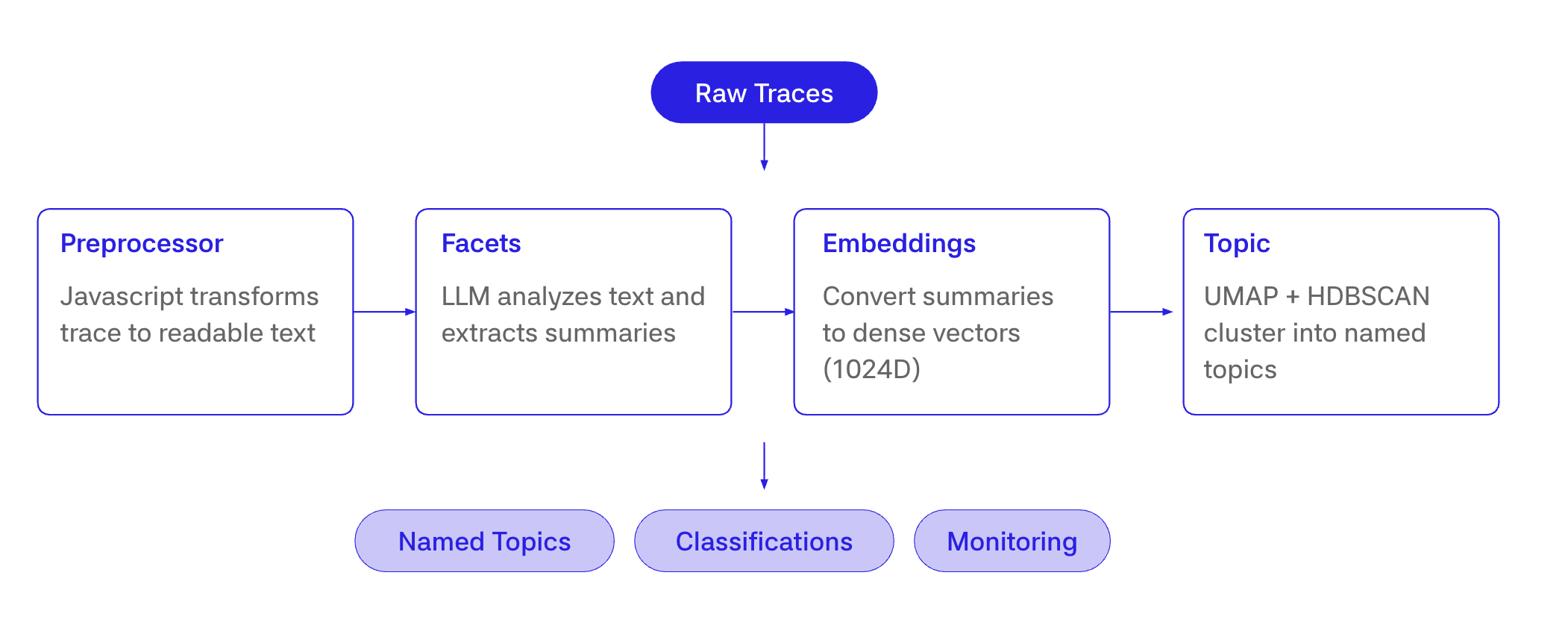
Stage 1, preprocess

The preprocessor turns a raw trace into tokens. The default preprocessor walks every span in scope, parses each span as an LLM conversation, deduplicates messages across spans, and drops scorer spans. Custom preprocessors are JavaScript functions that return text, an array of text, or null to skip the trace. These are easy for humans or LLMs to write, because they just move around the data in a span to a desired format.

This stage exists for one reason. Raw traces can be enormous, and the facet model has a finite context window. Preprocessing typically runs in well under a second per trace, and the output is hard-capped at 128K tokens before it ever reaches the facet model. It's also the biggest place we depart from Clio. Clio summarizes conversations that already arrive in a roughly uniform shape, while we have to turn arbitrary, sprawling agent traces into something a single LLM pass can handle.

Stage 2, facet extraction

The facet stage is where the LLM does its one job. Each facet has a prompt, like "summarize what the user is trying to accomplish in one sentence," and an output schema. The facet model produces a short text blob, typically a sentence or two, and writes it back to the trace as facets.<FacetName>.

The built-in facets are Task, Sentiment, and Issues. Custom facets are user-defined prompts that can be anything from use case to SKU segmentation.

There's one optimization in this stage that matters a lot for cost. A naive implementation would compute facets one at a time, so running five facets on a trace would cost roughly five times the trace tokens plus five facet prompts. Prompt caching can take some of that off, but it's much harder to get right and still expensive at this volume. We batch facets into a single LLM call, so the cost is [trace tokens] + [# facets] × [facet prompt tokens]. Trace tokens are paid once regardless of how many facets you run. Five facets is not five times more expensive than one.

The facet model is a Braintrust-managed model served on Baseten. We're currently using Gemma because it performed the best compared to other small models. Each facet run takes around 10 seconds on average. Because we run them in asynchronous batches, it can take up to 60 seconds during spikes, which is fine for a continuous background pipeline.

Stage 3, embedding

After the facet text is produced, we embed it with our embedding model, also served on Baseten. The output is a 1024-dimensional dense vector.

The thing to notice here is what we're embedding. It's the facet output, not the raw trace. That's what makes the rest of the pipeline tractable. A consistent, short, on-topic summary embeds cleanly. A million-token agent trace does not.

The vector is stored in Brainstore alongside the facet text on the trace and is garbage-collected on the project's retention schedule.

Stage 4, clustering

Once enough facet embeddings have accumulated, the clustering stage runs on a sample of up to 50,000 facets per generation pass. The default algorithm is HDBSCAN with UMAP for dimensionality reduction. K-Means and Hierarchical are available as alternative clustering algorithms, and PCA is available as an alternative dimensionality reduction.

We picked HDBSCAN as the default for two reasons. It doesn't require you to pick the number of clusters up front, which matters because the right number of topics is a function of your data and changes over time. And it naturally identifies outliers as noise rather than forcing every point into a cluster, which lines up with the way real traffic distributes, namely a long tail of one-off requests around a small number of recurring patterns.

For keyword extraction per cluster we use c-TF-IDF, which is the same approach BERTopic popularized. A generation pass over thousands of traces completes in roughly 30 seconds. Around 10 seconds of that is clustering, which is written in Rust. The rest is a series of LLM calls to name the clusters.

Stage 5, naming

The naming stage takes the representative facet exemplars for each cluster and asks an LLM to produce a short name and description. This is generative, which means the same cluster can pick up a slightly different name on the next generation pass even if the underlying membership barely changes. One of the big learnings was that you have to use a large model and name multiple clusters simultaneously, otherwise the names are not very discriminative. That's why we treat the cluster, not the name, as the stable identity. When a new topic map is generated, we automatically match similar clusters to their predecessors and reuse their ids.

Stage 6, classification

Classification is the cheap part. For each new trace, we run the preprocess, facet, and embed stages, then look up the nearest cluster centroid in the saved topic map. If the trace is within the configured distance threshold, it gets a label. If it's not, we write no_match instead of forcing a bad label.

No LLM call happens at classification time. The whole step is around 100 milliseconds per trace, which is what makes it possible to run on 100% of traffic after sampling.

The result lands on the trace as classifications.<TopicMap>[0].label, alongside the embedding distance and the cluster index as metadata. From that point on it behaves like any other column in your logs. You can filter on it, group by it, join across topic maps, or query it from SQL.

SELECT
  classifications.Task[0].label as topic,
  count(*) as count
FROM project_logs('my-project-id')
WHERE classifications.Task IS NOT NULL
  AND created > now() - interval 7 day
GROUP BY topic
ORDER BY count DESC

That SQL pattern is what we mean when we say Topics outputs are queryable. The classification lands as a column on the trace, which means you can filter on it, group by it, alert on it, or join it with anything else in your logs. The full query patterns are documented in the SQL reference.

The automation that ties it together

The other half of Topics is the automation layer that runs the pipeline continuously, in the background, with sensible defaults and the right state machine.

A topic automation is a small state machine that moves through four states. It starts in waiting_for_facets, where it accumulates facet data. Once enough data is there, it transitions to recomputing_topic_maps, runs the cluster generation pass, and produces a new topic map. From there it moves to a backfill state, which classifies recent traces with the new topic map, and finally settles into idle until the next scheduled run.

There are two thresholds worth knowing about. You need at least 400 traces in a project for Topics to start, and at least 100 unique facet summaries before it will generate a topic map. Below those numbers, the clusters aren't meaningful and we'd rather show you nothing than show you noise.

Daily topics versus ad-hoc clustering

There are two places in the product where you'll see clusters.

The Topics view shows the automated topic map. The same persistent set of clusters, the same names, applied consistently to your logs over time. This is what you want for trend dashboards, alerting, and any analysis that needs to be comparable across days or weeks.

The "Cluster traces by facet" action on a filtered view runs ad-hoc clustering on whatever subset you're currently looking at, with parameters tuned for exploration. The clusters you get are specific to that slice. Run it on yesterday's failures, on a specific user cohort, on a single experiment. This is what you want when you're investigating, not monitoring.

Both views use the same pipeline. The difference is whether the topic map is persisted and reused or generated on the fly.

Models, hosting, and data flow

All native Topics inference runs on Baseten. That covers facet extraction, embedding generation, and topic naming. Baseten operates on zero data retention for inference payloads, so the inputs and outputs we send for inference are not stored.

We're deliberate about what gets sent. The facet model sees preprocessed text, which is itself capped at 128K tokens and stripped of attachments and metrics. The embedding model only ever sees the facet output, never the raw trace. The clustering step operates on embeddings and facet outputs, never on raw trace contents.

Topics inference can be hosted in both the US and EU, and we're HIPAA compliant. In BYOC deployments, your trace data stays in your data plane, and Topics native model calls egress to Baseten. Org admins can disable native models entirely, which turns Topics off across the org.

Topics runs on native models by default. The facet step is intentionally turnkey because that's where most of the quality engineering lives, and the prompt is co-tuned with the model. For naming, you can use your choice of models.

Architecture as developer experience

The architectural choices above translate into a few concrete properties you'll feel as a developer.

The pipeline runs continuously rather than as a batch job. Classification is embedding-only and runs on every matching trace as it arrives. Topic maps regenerate daily by default, with a configurable cadence. You don't kick off a job, you don't wait for a nightly run, and the labels you see on a trace are caught up to within minutes of ingestion in most projects.

Outputs are queryable, not just available in the UI. Classifications live on the trace as a structured column and are reachable from SQL. The topic for a trace is a WHERE clause you can build on, alert on, or join with other facets to answer questions like "what are the top tasks where sentiment is negative this week."

One pipeline serves every dimension you care about. Adding a custom facet doesn't mean wiring up new clustering, new naming, or new classification. The downstream stages don't care what dimension you're extracting along. The cost of a new facet is the cost of a prompt and the marginal cost of the facet prompt tokens, with no new pipeline behind it.

Identity stays stable across regenerations. Topic maps regenerate, names drift, but the underlying cluster identity is matched across runs so your dashboards and saved queries keep working. The thing you depend on, the cluster, is stable. The thing that can drift, the name, is treated as a label.

Topics is batteries-included, and the escape hatches are there when you need them. The built-in facets and the default preprocessor are designed for most projects out of the box. When your trace shape is unusual, like a multi-agent setup where the default thread preprocessor pulls in too much scorer output, you can drop in a custom JavaScript preprocessor that returns exactly the spans you want clustered on. The full pipeline behind it is the same.

If you want to see the surface area in more detail, the Topics documentation covers the product, custom facets walks through writing your own facets, and managing Topics covers the automation controls. The SQL patterns for working with classifications are in the SQL reference.

Topics is the second of the bets we've talked about publicly, and like Brainstore it has only gotten more useful as our product has grown. We think of it as the most universal baseline layer of intelligence you can run, cheap enough to apply to 100% of your traces. The more expensive and more powerful layers we're building sit on top of that baseline. The team behind it is small, the surface area is bigger than it looks, and we think the pipeline shape is going to continue to be useful as production AI workloads keep getting more complex.